
Table of contents
2. Data basis
2.1. Spatial reference units
The study was built on the ‘European catchments and rivers network system’ (Ecrins), i.e. a geographical information system of the European hydrographical sub-catchments organised from a layer of 104,684 so-called ‘Functional Elementary Catchments’ (FECs) with an average size of about 60 km2 (EEA, 2012). The FEC-level represents the spatial unit at which all data used in this study were processed. All data referring to different spatial units (e.g. NUTS or E-HYPE sub-basins) were transferred into FEC-level (see Globevnik et al., 2017).
2.2. Existing landscape classifications
Two existing landscape classifications were influential to this study: (1) Six different agricultural land systems (derived from the “Land-system Archetypes” of Levers et al., 2018) and (2) four major European agricultural regions (derived from the biogeographical regions of the Habitats Directive of the European Community; Roekaerts, 2002).
The “Land-system Archetypes” developed by Levers et al. (2018) were defined at the pan-European scale (covering EU-28, except Croatia) on the basis of selected land-use indicators (e.g. various agricultural or forestry land cover, fallow farmland, nitrogen input, livestock density) representing the conditions in the year 2006. These archetypes describe landscapes featuring similar patterns of land cover and management intensities related to farming and forestry. Management intensity is classified by indicators of input-intensity (nitrogen application rates, livestock stocking densities) and output-intensity (amount of harvested biomass). The “Land-system Archetypes” were aggregated into six agricultural land systems characterised by type of land cover and management intensity: intensive and extensive cropland, intensive and extensive livestock, extensive grassland and fallow farmland. Management intensity classifies the material and labour input and harvest yield output, generally separating between intensive and extensive agricultural land systems.
Four major European agricultural regions were delineated to be used in all subsequent analysis: Western, Eastern, Mediterranean, and a combination of Northern and Highlands. This classification is framed by the biogeographical regions in Europe (Roekaerts, 2002) grouped into four major regions matching the geographical intercalibration groups relevant in ecological freshwater status assessment (Poikane et al., 2014). It considers the coarse climatic and socio-economic differences between the areas, which influence the agricultural land systems: The Western area generally exhibits favourable climatic and economic conditions for productive agriculture, while the Eastern area is still characterised by less-favourable conditions for historically and socio-economic reasons. Climate-induced water scarcity is the decisive factor in the Mediterranean, and the Northern and Highland areas are largely less-favourable areas for agricultural production due to wet and cold climatic conditions (Metzger et al., 2005; Kuemmerle et al., 2008).
Figure 2 shows the distribution of different agricultural land systems across Europe, for which the management intensity was quantified combining nitrogen input, livestock density and harvested output (Levers et al., 2018), together with the major agricultural regions of Europe.
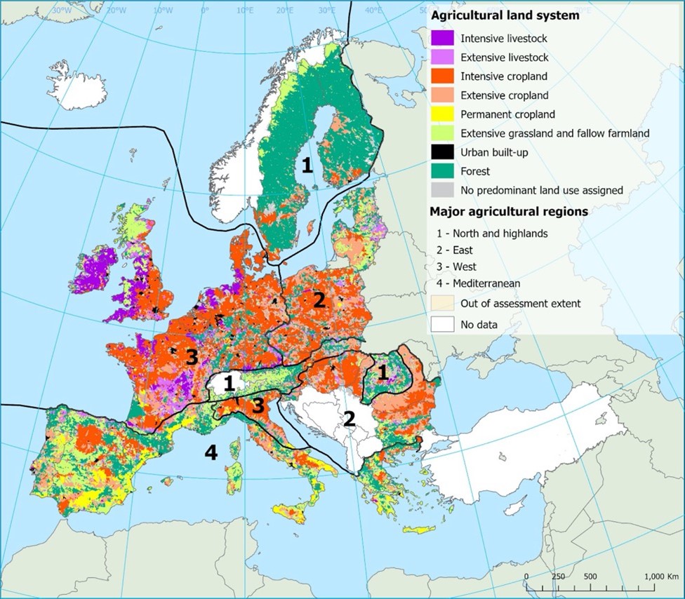
Figure 2: Agricultural land systems distributed across four major agricultural regions in Europe. The map shows the dominant land system per FEC (see text for details).
2.3. Pressure data
Pan-European data sets on agricultural pressures were developed based on available modelled or remotely sensed datasets. These datasets include diffuse pressures (nutrients, pesticides), hydrological pressures (water abstracted for irrigation) and agricultural land use in the river floodplain (proxy-indicator for various direct agricultural pressures including morphological alteration). The available data are specified in the following sections.
Note: All pressure data used met the criteria of being available on pan-European scale at a spatial resolution corresponding to the FEC-level. Aspects of data accuracy and uncertainty have not been specified in this document, as this consultation primarily aims at learning your views on the overall approach of defining a composite multi-pressure index on water from agriculture.
Diffuse pressures: nutrients
To estimate the effects of farming-related nutrient pollution on freshwater ecosystems, the parameter nitrogen surplus, which is the difference between nitrogen input (e.g. fertilisers, feed) and output (e.g. animal and plant products), was used. It was calculated using the CAPRI (Common Agricultural Policy Regional Impact Analysis) modelling system (Britz and Witzke, 2014), a global economic model for agriculture with a regionalised focus for Europe, which uses regional and national data inputs based on official EUROSTAT statistics. The CAPRI nitrogen balances relevant for this study were estimated for the year 2012, on the basis of four components:
- Export of nutrients by harvested material per crop, depending on regional crop patterns and yields,
- output of manure, depending on the animal type,
- input of mineral fertilizers, based on national statistics at sectoral level and
- a model for ammonia pathways. The model outputs provided indicators of regional farm, land and soil nitrogen-budgets and nitrogen-flows of the agricultural sector at the European scale (Leip et al., 2011).
The indicator ‘nitrogen surplus on agricultural areas’ was selected as a proxy for nutrient pollution pressure, aggregated at FEC-level (Figure 3).
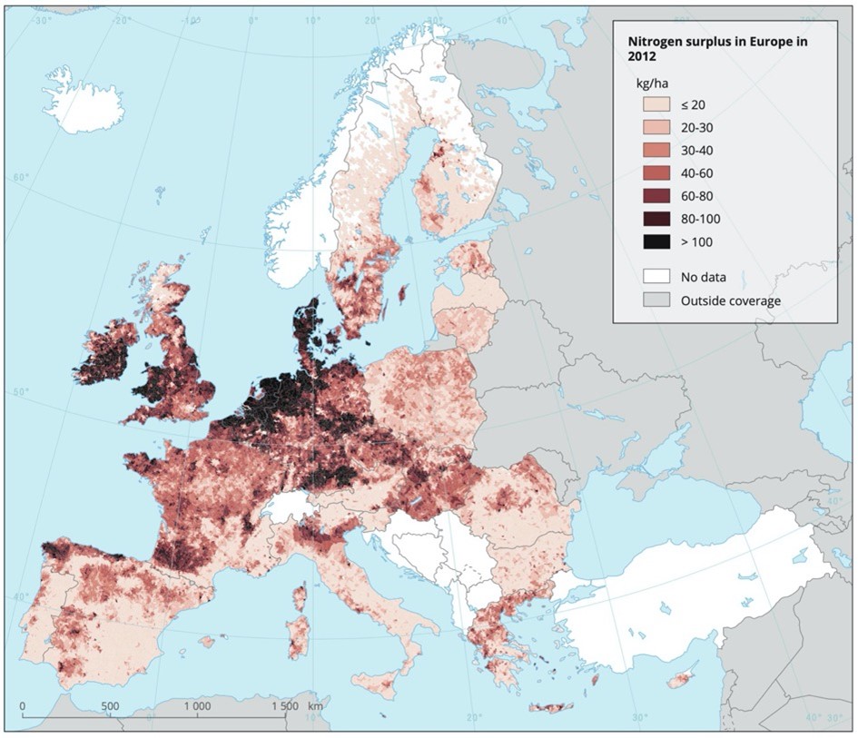
Figure 3: Geographical distribution of the nitrogen surplus on agricultural areas, calculated by FEC
Diffuse pressures: pesticides
To quantify the effects of pesticides on the freshwater ecosystems, he chronic multi-substance Potentially Affected Fraction (msPAF) was used, derived from Europe-wide integrated exposure and effect modelling for the year 2013 (van Gils et al., 2020). The msPAF specifies the potential share of the aquatic species community affected by pesticide toxicity. The model includes two components:
(1) a spatio-temporally resolved model for emissions and fate-transport of chemicals driven by a hydrological model (van Gils et al., 2020), yielding Europe-wide daily predicted environmental concentrations (freely dissolved part) of 332 pesticides in water bodies to obtain a “real-life” mixture exposure scenario for each FEC, and
(2) species sensitivity distributions (SSD) based on effect models considering chronic non-observed-effect concentrations (NOEC) of each studied chemical as effect endpoint (Posthuma et al., 2019). Combining (1) and (2), and adding a step of mixture modelling yields the mixture toxic pressure metric, which is expressed as multi substance Potentially Affected Fraction of species (msPAF) (de Zwart & Posthuma, 2005; Posthuma et al., 2020), being an estimate of the likelihood (values between 0 and 1) of direct effects of chemical exposure to effect-endpoints of aquatic organisms such as growth and reproduction (Posthuma et al., 2019). In this study, the msPAF-NOEC based on 99th percentile predicted environmental concentrations of the daily concentration estimates was used, representing an acute toxic stress level exceeded at four days per year (Figure 4).
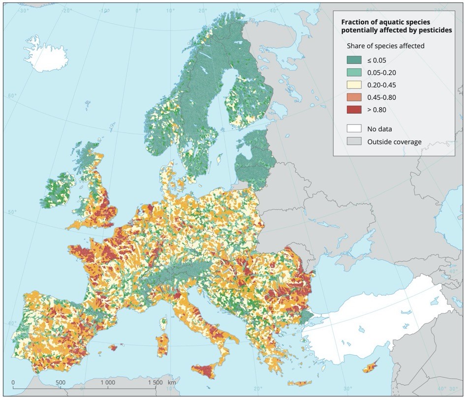
Figure 4: Geographical distribution of the fraction of aquatic species in Europe potentially affected by pesticides, calculated by FEC
-
From AGRI: The inland of Sicily seems to be concerned, but that area is composed by extensive agriculture, grazing area. It is impossible there is pressure on aquatic species. That is a mountain area.
-
It´s unknown what baseline data was used and what methodology was applied
In this theme 332 pesticides are referred, but none are mentioned as examples, so it is not clear the methodology adopted.
Hydrological pressure: water abstracted for irrigation
To consider the effect of crop irrigation, the annual volume of water abstracted for agricultural irrigation (acquired for the year 2015) was compiled (Zal et al., 2017). Water abstraction represents the main driver of water consumption in agriculture. The data are intermediate model outputs from pan-European water quantity accounting at FEC-level with monthly resolution. The monthly values were summed up to the total annual amounts and transformed to cubic metres per hectare, dividing the annual water abstracted in each FEC by the irrigated crop area in the respective FEC (Figure 5).
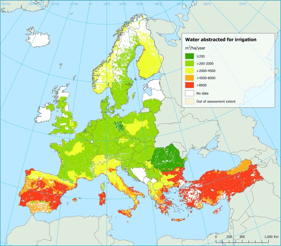
Figure 5: Geographical distribution of the annual volume of water abstracted for agricultural irrigation, calculated by FEC
-
Portugal appears to have a high water consumption compared to other countries, but it is not possible to validate the results shown on this map because it is unknown what baseline data was used and what methodology was applied.
-
Comment from Austria: The information in Figure 5 is not optimal for Austria. Irrigation is only responsible for a very minor (4%) share of water abstraction and located in very small parts of the country. But Austria in total falls, inspite of the small-scale resolution, ino category >200-2000 m³/ha/year water abstraction for agricultural irrigation. This is not a big number, however it is not representative for the whole territory.
Agricultural land use in potential river floodplain
To incorporate the hydromorphological alteration caused by agriculture, the area of agricultural land located in the potentially flood-prone areas was calculated as an average of the years 2011 to 2013 (EEA, 2020; Figure 6). It was derived from two spatial layers, (1) the JRC flood hazard map for Europe 100- year return period, compiled with the flood model ‘LisFlood’ (Bates & De Roo, 2000; Alfieri et al., 2014) and (2) the Copernicus Potential Riparian Zone layer compiled with data from the Copernicus Land Monitoring Service (EEA, 2015; CLMS, 2019). This proxy-indicator allows for an estimate of various farming-related pressures on the freshwater ecosystems and can be interpreted as the probability of morphological alterations to surface waters due to agricultural activities, e.g. drainage of floodplain area caused by agricultural production.
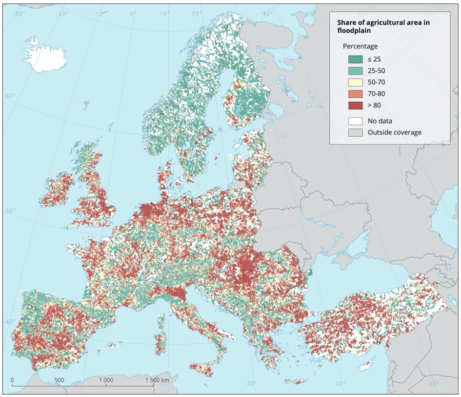
Figure 6: Geographical distribution of the share of agricultural land in floodplain areas, calculated by FEC
The main pressure resulting from agriculture are the nutrients, nitrogen and phosphorous. In this theme the phosphorus is not covered but we consider it should be included.